How to Implement Reinforcement Learning Without Temporal Difference Learning: A Divide-and-Conquer Approach

Introduction

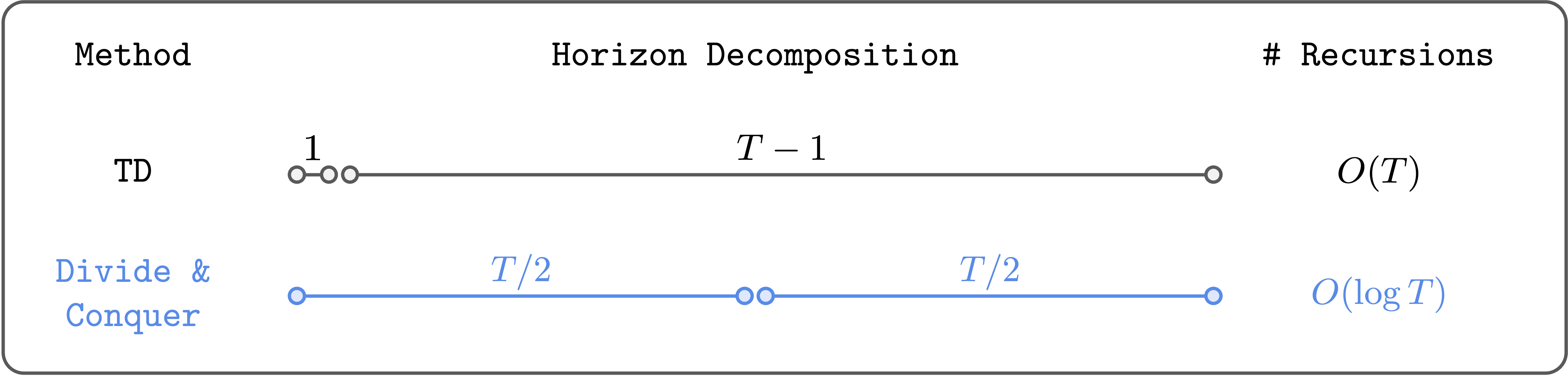
Reinforcement learning (RL) traditionally relies on temporal difference (TD) learning to update value functions, but this bootstrapping can cause error accumulation in long-horizon tasks. This guide presents an alternative approach: divide-and-conquer RL that sidesteps TD learning entirely using Monte Carlo returns. By breaking a complex task into manageable subproblems, you can achieve scalable off-policy learning without the compounding errors of bootstrapping. Follow these steps to implement your own non-TD RL algorithm.

What You Need

• Environment: A Markov decision process (MDP) with a long horizon or sparse rewards.
• Off-policy dataset: Pre-collected experience tuples (state, action, reward, next_state) – can include old policies, human demonstrations, or internet data.
• Programming tools: Python with NumPy, and a deep learning framework (PyTorch or TensorFlow) for function approximation.
• Basic RL knowledge: Understanding of value functions, policy evaluation, and Monte Carlo methods.
• Divide-and-conquer blueprint: A predefined way to split the horizon into subtasks (e.g., subgoals, options, or fixed-length segments).

Step-by-Step Instructions

Step 1: Decompose the Task into Subtasks

Identify natural breakpoints in the task – either by domain knowledge (e.g., subgoals like “reach door” in a navigation task) or by fixed-length intervals. For example, if your task has a horizon of 1000 steps, split it into ten 100-step segments. Each subtask becomes a smaller MDP with its own start and terminal states. This division is the core of the divide-and-conquer paradigm: you will solve each subtask independently using pure Monte Carlo returns, avoiding TD bootstrapping across the whole horizon.

Step 2: Collect Off-Policy Data for Each Subtask

Use your existing off-policy dataset. For each episode, extract the experience trajectory that falls within a given subtask. If you split by time, simply slice the episode into fixed-length chunks. If you use semantic subgoals, filter transitions where the state satisfies the subgoal condition. Ensure you have multiple trajectories per subtask from diverse policies – this off-policy flexibility is the main advantage of this method. Label rewards within each subtask as if the subtask were an independent episode (discount within the subtask, but do not carry value across subtask boundaries).

Step 3: Estimate Subtask Returns Using Monte Carlo

For each subtask, compute the Monte Carlo return for every visited state-action pair. Use the raw discounted sum of rewards from that point until the end of the subtask (no bootstrapping). This is equivalent to setting n equal to the subtask length in n-step TD, but crucially you never propagate values from one subtask to another. The formula:
\( G_t = \sum_{k=t}^{T_{sub}} \gamma^{k-t} r_k \)
where \(T_{sub}\) is the subtask terminal step. This eliminates error accumulation across subtasks. Store these Monte Carlo returns as targets for value function training.

Step 4: Train a Value Function for Each Subtask (or a Universal One)

Train a value function (Q-function or V-function) per subtask to predict the Monte Carlo returns. You can maintain separate neural networks for each subtask, or a single network conditioned on a subtask identifier (e.g., one-hot vector or goal embedding). Use supervised learning with mean squared error between predicted value and Monte Carlo return. Because there is no bootstrapping, you avoid the divergence issues common in off-policy TD. The training can be entirely offline using your collected data, making it sample-efficient.

Step 5: Combine Subtask Values for Action Selection

At decision time, the agent selects actions by evaluating all subtask value functions (or the universal one) for the current state. However, to make a global decision, you need to stitch subtask values together. A simple approach: treat each subtask as an option and use the value of the subtask plus a planning routine to choose which subtask to pursue. Alternatively, if subtasks are disjoint, run the first subtask until termination, then switch to the next. For more sophisticated integration, compute an overall value as a sum of subtask values adjusted by a discount factor between subtasks – but avoid bootstrapping across subtasks to stay true to the no-TD philosophy.

Step 6: Iterate and Refine Subtask Boundaries

After initial training, evaluate performance on the full task. If the agent fails, consider adjusting the subtask decomposition: make segments shorter to reduce Monte Carlo variance, or realign boundaries to natural state transitions. Because you are not backpropagating errors across subtasks, this refinement is stable – you can retrain subtask value functions independently without affecting others. You may also discover that some subtasks need more data or a different discount factor. Repeat steps 2-5 until the full-horizon performance is satisfactory.

Tips for Success

• Choose subtask lengths wisely: Shorter subtasks yield lower Monte Carlo variance but require more subtasks and more computation. Longer subtasks reduce the number of subtasks but increase variance. A good rule of thumb is to aim for subtask horizons where the return variance is manageable (e.g., 50-200 steps).
• Exploit off-policy data diversity: Since you don’t need fresh on-policy data, curate a dataset that covers diverse behaviors within each subtask. This boosts generalization and prevents overfitting to narrow experiences.
• Avoid implicit bootstrapping: When combining subtask values, resist the temptation to use adjacent subtask values as targets for the previous subtask – that would reintroduce TD-style error propagation. Keep subtask training completely independent.
• Use discounting only within subtasks: Set the discount factor \(\gamma\) to reward immediate subtask completion. The overall task discount can be handled by the ordering of subtasks (if sequential) or by a separate planning layer.
• Test with simple gridworlds first: Before deploying on complex continuous control, verify the algorithm in a domain where you can visualize subtask boundaries and value predictions.